Tutorial¶

Analysis of data from a calibration run involves three main steps:

Reading in transmitter position data and receiver spectrum
Interpolating receiver spectrum to drone flight times
Gridding data onto a healpix map

A mapping run is split into smaller chunks of flight aka ‘sorties’ owing to the battery life of the drone. Each of these sorties is associated with a transmitter position file and a receiver spectrum.

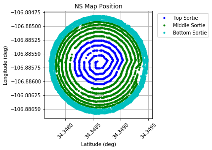
2D plot of a hemispherical flight pattern.¶

Reading in transmitter position data¶

Transmitter position is derived from drone logs. These logs come in two data formats: tlog and ulog format.

Tlogs are telemetry logs recorded by the ground station when the drone is powered on and connected.
Ulogs are position logs saved on the drone’s SD card.

Two functions read_tlog_txt and read_ulog are available on ECHO.readutils to extract transmitter position data from these log files.

Reading in receiver spectrum¶

Data formats of receiver spectrum files may vary with the telescope but usually, it is a hdf5 file containing spectra vs time.

Receiver spectrum files can be read-in using read_h5 function from ECHO.readutils.

Matching up receiver spectrum with drone flight times¶

We begin with instantiating an Observation Object and pass in coordinates of antenna under test (AUT), programmed frequency of transmitter in MHz and a short description of AUT

import ECHO

NS_Obs = ECHO.Observation(lat=34.3486, lon=-106.8857, frequency=70, description='LWA Antenna 137')

We define paths to the files associated with each sortie :

datadir = '/LWA_October_2019/data/'

NS_Obs.addSortie(
    tlog=datadir+"tlog_data/NSMap_MiddleSortie.txt",
    ulog=datadir+"ulog_data/NSMap_MiddleSortie.ulg",
    data=datadir+"LWA_spectra/NS_Sorties/01_NSmap_MidSortie_waterfall.hdf5",
    sortie_title="NS Mid"
    )

To read these files, we call the read_sorties() function

NS_Obs.read_sorties()

The data is stored in dictionaries and can be accessed as :

print(NS_Obs.sortie_list[0].t_dict.keys())
print(NS_Obs.sortie_list[0].u_dict.keys())

Additional sorties can be added to a single observation using the addSortie() function

#add two additional sorties
NS_Obs.addSortie(
    tlog=datadir+"tlog_data/NSMap_TopSortie_Repeat.txt",
    ulog=datadir+"ulog_data/NSMap_TopSortie_Repeat.ulg",
    data=datadir+"LWA_spectra/NS_Sorties/03_NSmap_TopSortie_waterfall.hdf5"
    )

NS_Obs.addSortie(
    tlog=datadir+"tlog_data/NSMap_BottomSortie.txt",
    ulog=datadir+"ulog_data/NSMap_BottomSortie.ulg",
    data=datadir+"LWA_spectra/NS_Sorties/02_NSmap_BotSortie_waterfall.hdf5"
    )

#read in all of the current sorties, apply bootstart correction, and flag the start/endpoints
for sortie in NS_Obs.sortie_list:
    sortie.read() #Note that this replaces all previous reads
    sortie.apply_bootstart()
    sortie.flag_endpoints()

#takes the data from all sorties, sorts them by time, and combines them into a single array
NS_Obs.combine_sorties()

Matching up telescope data to drone positions¶

Telescopes record data at a higher rate than a gps module on the drone. To match up the telescope data to the drone positions, we downselect and interpolate telescope data.

#combine the drone position data with the intrument response
NS_Obs.interpolate_rx(1,1,'XX')

Gridding data¶

A common way to store beam models in 21cm pipelines is to use the HEALPix pixelization scheme. Hence, we’ll be gridding our data onto a healpix map.

To do so, we create a Beam object

NS_Obs.make_beam()

Once the beam object is created, the healpix map can be visualised by executing

NS_Obs.plot_beam()

Analysis¶

E and H planes of the beammap can be plotted by executing
```
NS_Obs.plot_slices(figsize=(10,10))
```
ECHO uses pyuvbeam to read-in CST export files of the transmitter beam.

To do so instantiate a Beam object with beam_type = ‘efield’ or ‘power’ and call the read_cst_beam():

tx_beam = ECHO.Beam(beam_type= 'efield')
CST_file = '../Chiropter_NS_PECBico_ff70_ZupYnull.txt'
tx_beam.read_cst_beam(CST_file, beam_type='efield', frequency=[70e6],
               telescope_name='Chiropter', feed_name='BicoLOG', feed_version='1.0',
               model_name = 'Chiropter_NS_2019', model_version='1.0', feed_pol='y')

To plot the cst beam:

tx_beam.plot_efield()